
Table of contents
- Scientific introduction
- The Lindblad model used in this demonstration
- Test progress
- Demo user request
- Demo data
- Installation and execution
- Results and artifacts
- Physical interpretation
- Reproducibility
- Common failure modes
- Limitations
- References
- Try this workflow
Scientific introduction
Open quantum systems exchange energy or information with an environment, so their evolution cannot generally be represented by a closed-system Schrödinger equation alone. A widely used Markovian description is the Lindblad master equation, which evolves a density operator under a Hamiltonian plus dissipative collapse terms. For a zero-temperature damped harmonic oscillator, a collapse operator proportional to the annihilation operator removes excitations. Starting from a Fock state with five photons, the expected mean photon number follows the analytic law n(t) = n0 exp(-κt) when the damping convention is chosen consistently.
This model is small enough to admit an exact expectation yet rich enough to test an open-system solver, operator construction, time-grid handling, steady-state analysis, structured export, and scientific visualization. The analytic curve acts as an independent reference for the numerical trajectory. Agreement does not prove that every open-system problem is correct; it demonstrates that one well-specified Lindblad calculation behaves as theory predicts under a pinned software environment.
QuTiP is a Python framework for simulating quantum systems, including state vectors, density matrices, operators, master-equation solvers, correlation functions, and steady states. The validated workflow uses QuTiP 5.0.1 with NumPy 1.26.4 and SciPy 1.11.4 on a Linux x86_64 CPU. No GPU or quantum hardware is involved. That environment choice is part of the result because binary compatibility between QuTiP, NumPy, and SciPy has caused real installation failures in older attempts.
The Lindblad model used in this demonstration
The truncated oscillator Hilbert space has dimension 20, comfortably above the initial Fock occupation of five. The annihilation operator a lowers occupation, the number operator is a†a, and the Hamiltonian is ωa†a with ω = 1. Zero-temperature loss is represented by one collapse operator sqrt(κ)a, where κ = 0.2. The initial state is |5〉, and the requested observable is the photon-number expectation from time zero through time 12.
The truncation deserves explicit attention. A finite-dimensional basis approximates an infinite harmonic oscillator. Because the system begins at occupation five and only loses excitations, dimension 20 provides ample headroom for this case. A driven or finite-temperature oscillator could populate higher levels and would require a convergence study over increasing Hilbert dimensions. The fact that one truncation works here is not a license to reuse it blindly.
mesolve integrates the master equation and returns expectation values on the requested time grid. The comparison curve is calculated directly from the input equation rather than fitted to the numerical data. This distinction prevents a weak circular test in which the expected curve is inferred from the same numerical trajectory it is meant to validate. The steady state is computed independently with QuTiP's steady-state solver; for zero-temperature damping and no drive, its photon-number expectation should be effectively zero.
Test progress
| Validation gate | Status | Retained evidence |
|---|---|---|
| Package transfer preflight | Passed | 13 distributions totaling 110,103,721 bytes |
| Managed package installation | Passed | QuTiP 5.0.1 environment retained locally |
| Native dynamics execution | Passed | mesolve, analytic comparison, and steady state |
| Real chat-directed execution | Passed | Agent loaded the skill and authored a managed-runner program |
| Semantic result validation | Passed | 121 rows, error tolerance, steady state, PNG and SVG checked |
| Focused publication capture | Passed | Results rendered inside the chat result surface |
Installation alone receives no scientific credit. The package probe confirms version and import health, then the native path establishes a deterministic reference. The separate chat path receives the scientific objective and JSON input, writes its own program, executes it through the skill-owned environment, and generates the requested artifacts. The harness examines actual tool messages to establish that the skill was loaded and the managed runner was used.
Demo user request
Use the installed
qutipskill anddamped-oscillator.jsonto simulate the specified zero-temperature open quantum system. Write and execute a task-specific Python program through the managed skill runner. Use QuTiPmesolvewith the stated Hamiltonian, Fock initial state, collapse operator, and photon-number observable; also compute the steady state. Createqutip-results.json,photon-decay.csv,photon-decay.png, andphoton-decay.svg. Compare every simulated point with the analytic exponential, report the maximum absolute error, verify the steady-state photon number, and summarize the physical result and output paths. Do not install another copy and do not fabricate values.
The prompt is deliberately written as a scientific request rather than a prepared program. It names the algorithmic requirements and deliverables but leaves the agent responsible for reading the skill, translating the JSON parameters into operators, writing executable code, invoking the managed runtime, and checking the real files. This is the behavior an E2E skill test must exercise.
Demo data
The complete input is damped-oscillator.json. It is compact, deterministic, and inspectable. The JSON states the Hilbert dimension, oscillator frequency, damping constant, initial Fock occupation, time interval, number of time points, analytic model, maximum accepted trajectory error, and steady-state tolerance.
| Parameter | Value | Role |
|---|---|---|
| Hilbert dimension | 20 | Finite basis used to represent the oscillator |
Oscillator frequency ω | 1.0 | Hamiltonian coefficient |
Damping constant κ | 0.2 | Zero-temperature photon-loss rate |
| Initial Fock state | 5 | Initial mean photon number |
| Time interval | 0 to 12 | Evolution window |
| Time points | 121 | Requested output grid |
| Analytic model | 5 exp(-0.2t) | Independent reference trajectory |
| Maximum absolute error | 0.02 | Numerical acceptance threshold |
| Steady-state tolerance | 1 × 10⁻8 | Acceptance threshold for vacuum occupation |
The time grid includes both endpoints, so the CSV validator requires exactly 121 rows, a first time of zero, and a final time of 12. It also checks that time, simulated value, and analytic value columns are present. These schema checks prevent a summary JSON from concealing an incomplete trajectory.
Installation and execution
The dependency transaction was downloaded into the per-skill retained cache before installation. The measured 110.1 MB transfer is safely below the strict 500 MB lightweight-host ceiling. A Python 3.11 environment is retained under the managed tool root, allowing future regression or failure repair without destroying the exact package state. The installed versions are intentionally pinned because QuTiP's compiled extensions must match the numerical Python stack.
python scripts/install.py
python scripts/tool.py probe
python scripts/tool.py run -- damped_oscillator_analysis.py
These commands expose the audited runtime boundary. In interactive use, a researcher does not need to write the analysis script: the scientific agent derives it from the chat request and input file. Showing the commands remains useful for reproducibility, environment diagnostics, and independent review.
The native reference and chat-authored programs follow the same scientific sequence: create destroy(N), build the number operator and Hamiltonian, create the initial Fock state, define sqrt(κ)a, generate the time grid, call mesolve, evaluate the analytic curve, calculate pointwise error, compute the steady state, and export both machine-readable and visual deliverables.
Results and artifacts
The chat-directed run produced 121 numerical time points. The maximum absolute difference between QuTiP's simulated photon-number expectation and 5 exp(-0.2t) was approximately 1.0872 × 10⁻10, far below the declared 0.02 threshold. The independently computed steady-state photon number was exactly 0.0 at the reported precision, satisfying the 1 × 10⁻8 tolerance.
| Result | Observed value | Acceptance rule | Status |
|---|---|---|---|
| Time rows | 121 | exactly 121 | Passed |
| First time | 0.0 | exactly 0.0 | Passed |
| Final time | 12.0 | exactly 12.0 | Passed |
| Maximum trajectory error | 1.0872 × 10⁻10 | ≤ 0.02 | Passed |
| Steady-state photon number | 0.0 | absolute value ≤ 1 × 10⁻8 | Passed |
| PNG dimensions | 2400 × 2400 | at least 500 × 300 | Passed |
| SVG content | substantive vector document | <svg> and >1,500 characters | Passed |
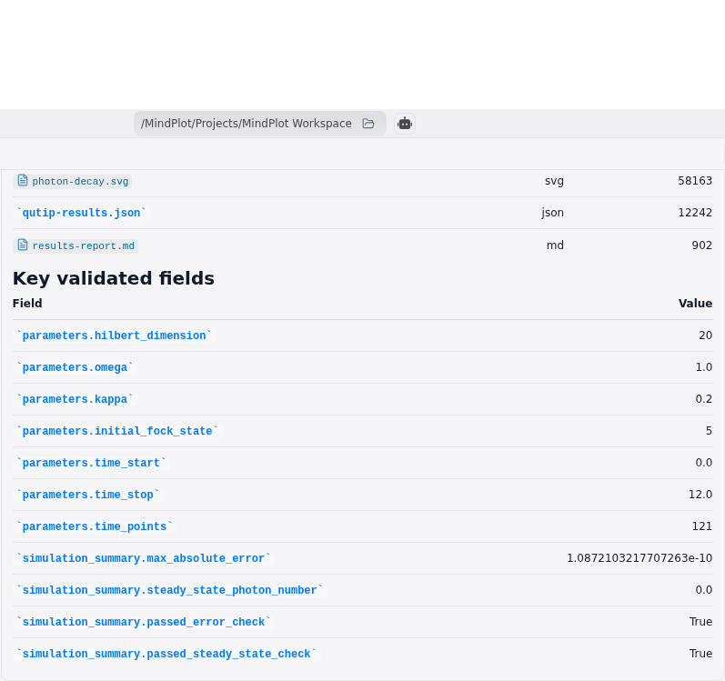
The focused capture emphasizes the scientific deliverables and validated scalar fields. It omits unrelated navigation, raw event streams, file lists, and oversized JSON displays. The underlying JSON and CSV remain the authoritative numerical sources.
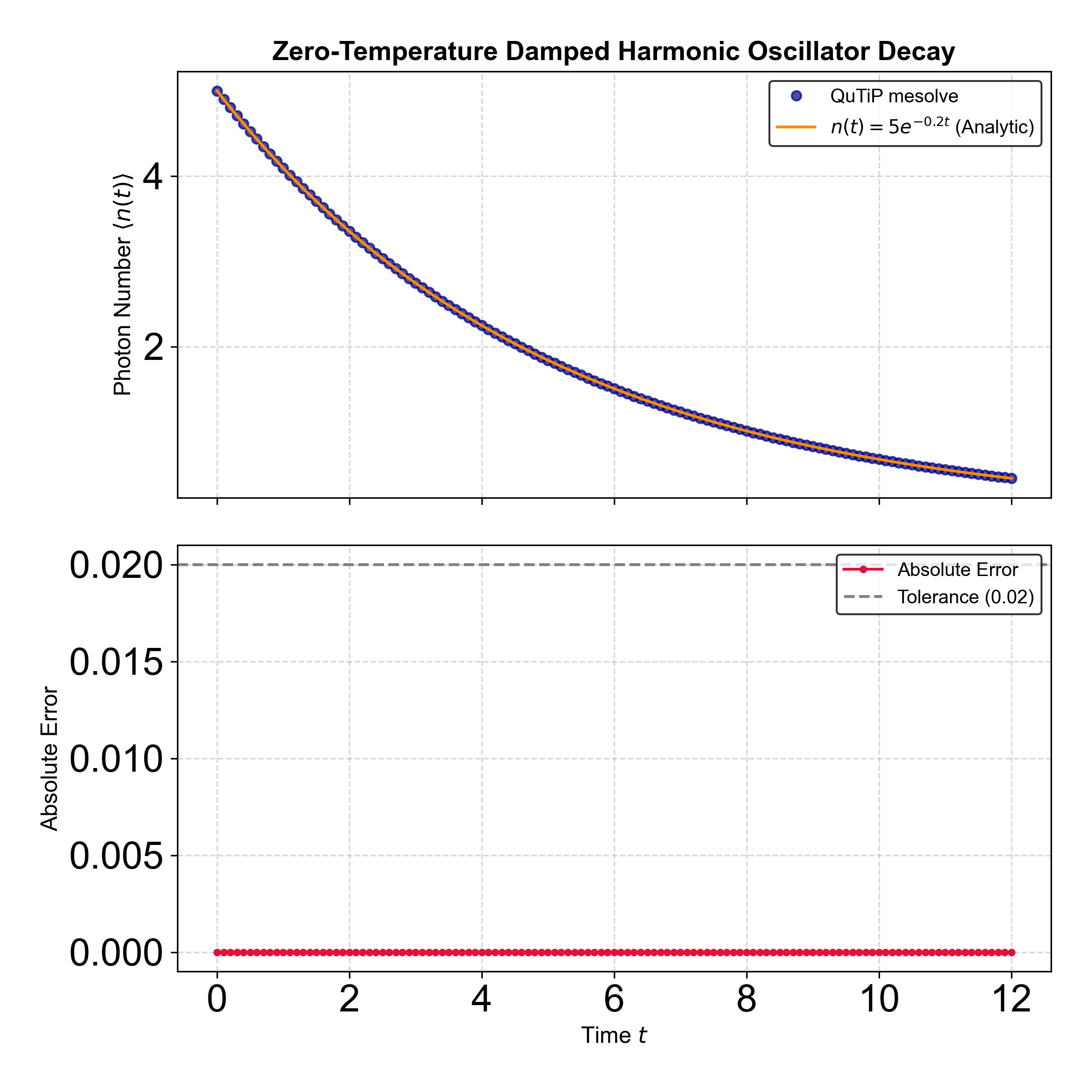
The plotted numerical and analytic curves overlap at the visible scale. Visual overlap is not used as the acceptance test; the row-by-row maximum absolute difference provides the quantitative check. The image is retained because it helps readers inspect monotonic decay, initial value, time range, labeling, and the absence of obvious oscillatory or sign errors.
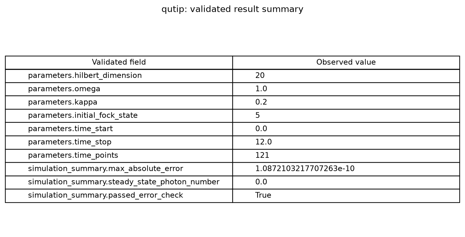
The summary visual is generated from retained structured artifacts and carries a provenance manifest with its source and digest. It is an explanatory view, not a replacement for raw data. This separation allows both accessible presentation and exact machine validation.
Physical interpretation
The result is consistent with exponential energy loss from an undriven oscillator into a zero-temperature Markovian bath. The initial expectation is five photons. As time increases, the collapse operator transfers population toward lower number states, and the mean occupation approaches vacuum. The stationary solution has zero photon number, matching the physical expectation for zero-temperature damping without a drive.
The tiny discrepancy from the analytic curve reflects numerical integration precision for this benign model, not experimental uncertainty. It should not be generalized to more demanding equations. Strong driving, time-dependent Hamiltonians, stiffness, non-Markovian environments, large Hilbert spaces, or near-degenerate Liouvillians can require solver-option studies and more careful convergence analysis.
The agreement also depends on using the same damping convention in the numerical and analytic models. Some texts define decay constants for amplitude while others quote an energy or occupation decay rate. A factor-of-two disagreement can therefore be a convention mismatch rather than a solver defect. Recording the explicit collapse operator and analytic equation removes that ambiguity.
Reproducibility
A complete reproduction should preserve the input JSON, package versions, Python ABI, operating system and architecture, generated program, exact output CSV, structured result JSON, and the validation report. The package cache and environment are retained locally. Publication images include cryptographic digests and source provenance, while the focused application screenshot is produced by Playwright against the actual result-rendering route.
Changing the solver version or numerical stack creates a new validation condition. The expected scientific curve remains the same, but numerical tolerances, default integrators, sparse-matrix behavior, or result-object schemas may change. A regression should compare semantics rather than assume byte-for-byte identity across versions.
For research beyond this demonstration, repeat calculations while increasing Hilbert dimension and tightening solver tolerances. Report convergence of the scientific observable, not merely command success. If stochastic trajectories replace the deterministic master equation, include multiple trajectories, random seeds, and uncertainty estimates.
Common failure modes
The most common installation risk is an incompatible compiled numerical stack. Pinning QuTiP without compatible NumPy and SciPy versions can produce import errors or runtime failures. The managed installer therefore treats the versions as one tested transaction. Network failures are mitigated by preserving downloaded wheels so a transient connection does not erase progress.
At the modeling level, errors include using κa instead of sqrt(κ)a, evolving a ket with collapse operators while misunderstanding density-matrix conversion, comparing amplitude decay to number decay, choosing a Hilbert space too small for occupied states, or reading the wrong expectation array. Output validators cannot infer every modeling intention, so the input contract and explicit operator description remain essential.
At the presentation level, a smooth plot may hide wrong units, an incorrect time endpoint, or a fitted reference curve. This workflow retains all 121 rows and calculates an independent analytic value for each time. The result only passes when the structured summary, tabular trajectory, and visual files agree.
Limitations
This is a zero-temperature, Markovian, undriven, single-mode demonstration. It does not validate finite-temperature baths, multiple collapse channels, driven dynamics, non-Markovian memory, quantum trajectories, correlation spectra, many-body systems, or experimental hardware. The analytic agreement validates the tested equation and environment, not the universal accuracy of QuTiP.
The measured package size and compatibility status apply to Linux x86_64 with Python 3.11. macOS, Windows, ARM, and CUDA were not validated in this run. The retained CPU pass should be displayed as such rather than converted into unsupported cross-platform claims.
References
- QuTiP documentation: dynamics and master equations
- QuTiP API: mesolve
- QuTiP documentation: steady-state solvers
- QuTiP 5 paper
- QuTiP original framework paper
Try this workflow
MindPlot includes built-in support for this scientific workflow. A researcher can describe the open-system simulation in natural language and attach the parameter file; the agent writes and runs the required code, preserves the numerical and visual deliverables, validates them, and explains the result. Try the web experience at mindplot.ai or download the desktop version for a more private local workflow and retained scientific environments.