
Table of contents
- Scientific introduction
- Test progress
- Demo user request
- Demo data
- Validated workflow
- Results and artifacts
- How to interpret the result
- Reproducibility
- Limitations
- References
- Try this workflow
Aeon provides a consistent Python toolkit for comparing, classifying, and clustering ordered signals without flattening away their temporal structure. In the worked example below, a DTW nearest-neighbor model identifies the direction of two unseen curves, time-series k-means recovers the two underlying trend groups, and distance measurements quantify why similar curves are treated differently from opposing ones. The two held-out predictions are correct; the DTW distance is 0.06 for two similar rising traces and 70.0 for a rising trace compared with a falling trace. These values make the example easy to audit, but the six deliberately simple curves are a software demonstration rather than evidence of accuracy on real-world data.
Scientific introduction
Why time-series learning needs specialized methods
A time series is an ordered sequence of observations indexed by time or another meaningful progression. Examples include electrocardiogram voltages, industrial vibration signals, astronomical light curves, environmental sensor measurements, longitudinal laboratory values, and transaction volumes. Ordering distinguishes these data from ordinary tabular rows. If the values are shuffled, the mean and variance may remain unchanged while the signal’s scientific meaning is destroyed. Useful analysis therefore needs representations and algorithms that respect temporal structure.
Time-series machine learning covers several distinct questions. Classification assigns an entire series to a known category. Regression predicts a continuous target from a series. Clustering discovers groups without supplied labels. Forecasting predicts future values from the observed past. Anomaly detection finds unusual points or subsequences. Segmentation locates changes between regimes, and similarity search retrieves related patterns. Aeon provides estimator-style interfaces for these tasks while following many conventions familiar from scikit-learn.
This demonstration focuses on three stable, inspectable capabilities: whole-series classification, whole-series clustering, and elastic distance measurement. The dataset is deliberately small enough that every value and assignment can be audited. Three traces rise from approximately zero to five, while three fall from approximately five to zero. Small offsets distinguish members within each group. The simplicity is useful for a software validation case because the scientifically expected relationship is explicit before the algorithm runs.
The example is not a benchmark. Perfect accuracy on two held-out synthetic traces says almost nothing about expected accuracy in a real application. It verifies that training labels, array orientation, distance calculations, predictions, cluster labels, and artifacts are connected correctly. A serious study would need representative sampling, a larger evaluation set, suitable preprocessing, uncertainty estimates, and comparisons with defensible baselines.
Dynamic time warping
Euclidean distance compares values at matching positions. It works when two signals are aligned and have comparable sampling. Real processes often progress at slightly different speeds: one heartbeat may be stretched, a gesture may be performed slowly, or a biological response may begin after a variable delay. Dynamic time warping, usually abbreviated DTW, compares two sequences while allowing a nonlinear alignment of their indices.
DTW constructs a cost matrix from pairwise differences and searches for a low-cost path from the beginning of both sequences to their ends. The path obeys monotonicity and continuity constraints so time does not run backward or jump arbitrarily. Its accumulated cost is the DTW distance. Warping can make the comparison robust to local timing variation, but unconstrained warping may also align unrelated events. Window constraints, normalization, derivative representations, and domain-specific preprocessing can materially change the result.
The retained values illustrate scale rather than universal thresholds. A1 and A2 have the same rising shape with an offset of 0.1 at each time point, giving a DTW distance of approximately 0.06 under the installed implementation and supplied representation. A1 and B1 move in opposing directions and give a distance of 70.0. The useful validated statement is that the within-pattern distance is far smaller than the across-pattern distance. Neither number should be transferred as a cutoff to another dataset.
Distance calculations are sensitive to units. A temperature series in degrees Celsius, a concentration series in micromoles per litre, and a normalized dimensionless trace have different scales. Multivariate series create an additional issue because high-variance channels can dominate. Analysts should document scaling, missing-value handling, resampling, filtering, and warping constraints. Those choices are part of the scientific method, not merely implementation details.
Nearest-neighbor time-series classification
The classifier used here is a one-nearest-neighbor estimator with DTW distance. During prediction, it finds the training series with the smallest DTW distance and returns that series’s class. This method is conceptually transparent: there is no hidden neural representation, and an analyst can inspect which training example determined a prediction. Nearest-neighbor methods with elastic distances are established baselines in time-series classification.
Four series were used for training: A1 and A2 labeled rising, and B1 and B2 labeled falling. The two withheld traces were A3 and B3. Aeon predicted A3 as rising and B3 as falling, producing two correct predictions and a demonstration accuracy of 1.0. The prediction CSV preserves expected and predicted labels rather than reporting only a scalar accuracy.
An accuracy of one from two cases has enormous uncertainty. A single error would reduce it to 0.5. The cases were designed to be easily separable and are not independent samples from a documented population. The result is therefore a deterministic regression target for the workflow, not evidence that DTW nearest neighbors will solve an applied classification problem. Real evaluation should include enough independent examples, class-specific metrics, confidence intervals, and a split strategy that prevents leakage between related subjects, devices, locations, or acquisition sessions.
Nearest-neighbor inference also scales with the number and length of stored training series. Approximate search, lower bounds, prototype selection, or alternative representations may be needed for large collections. Hyperparameters such as the warping window must be chosen using training data only. Selecting them after observing test performance leaks information and makes reported performance optimistic.
Time-series k-means clustering
Clustering asks whether series form useful groups without using the supplied class labels. Time-series k-means extends the familiar partitioning idea to three-dimensional collections of cases, channels, and time points. A distance and averaging strategy define how assignments and cluster centres are updated. With elastic distances, centre estimation can be more complex than taking a pointwise arithmetic mean.
The validated run requested two clusters and a fixed random seed. All A series received one cluster label and all B series received the other. Cluster identifiers themselves are arbitrary: label 0 does not intrinsically mean falling, and another valid initialization may swap 0 and 1. Semantic validation therefore checks membership relationships rather than exact numeric identifiers. It requires A1, A2, and A3 to share a cluster, B1, B2, and B3 to share another, and the two groups to differ.
The native test uncovered a real stability problem. With only two initializations, k-means could converge to an unhelpful local solution on this tiny dataset. Increasing n_init to ten while retaining a fixed random seed produced the expected separation reliably. This repair was added to the delivered instructions. It demonstrates why a successful process exit is not enough: a clustering command can finish normally while returning a scientifically poor partition.
In real exploratory work, the number of clusters is not known merely because an algorithm accepts n_clusters. Analysts may inspect stability across seeds and resamples, internal measures, cluster prototypes, and whether groups correspond to interpretable phenomena. Clustering can always divide data, but a partition is not automatically a discovery. Preprocessing choices, distance, representation, outliers, and sampling can dominate the result.
Array shape and data orientation
Aeon commonly represents a collection of equal-length univariate series as a three-dimensional array with shape (n_cases, n_channels, n_timepoints). The CSV stores one row per series with six time-point columns. The workflow converted six rows into an array of shape (6, 1, 6). Four training cases formed (4, 1, 6), while two held-out cases formed (2, 1, 6).
This orientation is an important validation target. Accidentally treating time points as independent samples would create six samples per trace and destroy the intended whole-series task. Reversing channels and time can sometimes produce code that runs but answers a different question. The summary records all three shapes so reviewers can verify that whole traces, not individual observations, were classified.
Unequal-length collections may use other Aeon-supported representations, and multivariate data increase the channel dimension. Analysts should consult the installed version’s API because experimental modules and accepted data containers can change. Schema validation should occur before fitting, with explicit checks for finite values, consistent units, label domains, sample identity, and leakage.
Reproducibility and package isolation
The package was installed into a retained skill-owned Python environment rather than the application’s controller runtime or a user’s global site-packages. A bounded preflight downloaded the exact Aeon 1.5.0 wheel and its core dependencies before offline installation. The complete transfer was 142,578,750 bytes, safely below the 500,000,000-byte lightweight-test ceiling. The installer records the version, Python version, transfer bytes, and cap in a manifest.
Core installation is intentionally different from installing every optional extra. Aeon’s optional dependencies cover additional estimators and deep-learning functionality, and they can greatly expand the environment. This test claims only the APIs it executed. It does not imply that every optional forecasting, anomaly-detection, segmentation, similarity-search, visualization, or neural estimator dependency has been installed and validated.
The first chat-driven attempt produced scientifically correct artifacts but used equivalent field names that the initial validator did not accept, such as true_label instead of expected. The test remained failed. The validator was repaired to check scientific meaning across documented aliases: expected and predicted labels must agree, cluster memberships must express the correct grouping, within-pattern distance must be smaller than across-pattern distance, the version must be exact, and the SVG must contain all six traces. A fresh chat attempt then passed. Retaining both attempts distinguishes a real rerun from retrospective relabeling.
Test progress
| Gate | Status | Retained evidence |
|---|---|---|
| Skill Hub installation | Passed | Installed skill copy and context view |
| Package preflight | Passed | 142,578,750 bytes, below 500 MB |
| Package installation | Passed | Aeon 1.5.0, Python 3.11.15 |
| Native feature execution | Passed after clustering repair | Classification, clustering, and DTW |
| Natural-language execution | Passed on attempt 5 | Configured chat runtime |
| Artifact validation | Passed | CSV, JSON, and SVG semantic checks |
| Platform | Validated | Linux x86_64 CPU; no CUDA required |
| Publication gate | Passed | Focused result screenshot and provenance manifests |
Demo user request
Analyze the six short time series in
data/time-series.csvwith the installed aeon skill. Use the skill-owned aeon 1.5.0 environment. Train a deterministic 1-nearest-neighbor DTW classifier on A1, A2, B1, and B2, then predict A3 and B3. Cluster all six series into two groups with deterministic time-series k-means, and compare the DTW distance between A1/A2 with A1/B1. Saveaeon-predictions.csv,aeon-summary.json, and a focusedaeon-series.svgshowing both trend groups. Report the package version, shapes, accuracy, cluster labels, both distances, and scientific limitations. Do not substitute generic sequence statistics or fabricate results.
The request is conversational rather than a prewritten program. The workflow had to identify the correct package environment, read the supplied CSV, preserve whole-series shape, run the specified algorithms, create three deliverables, and explain the interpretation boundary.
Demo data
The tracked time-series CSV contains six univariate traces and no private or externally sourced records. Each row has an identifier, a known demonstration label, and six ordered numeric values.
| Group | Series | Pattern | Role |
|---|---|---|---|
| Rising | A1, A2 | Training examples | DTW classification and distance reference |
| Rising | A3 | Held-out example | Expected prediction: rising |
| Falling | B1, B2 | Training examples | DTW classification |
| Falling | B3 | Held-out example | Expected prediction: falling |
The labels provide a test oracle for classification and help audit clustering after the unsupervised algorithm finishes. They should not be confused with a population-derived ground truth. The six traces were designed for deterministic software validation.
Validated workflow
The workflow parsed the six time columns as floating-point values, formed the Aeon collection shape (6, 1, 6), and selected four training and two test cases by identifier. It fitted KNeighborsTimeSeriesClassifier with one neighbor and DTW distance, predicted the held-out cases, and calculated exact accuracy.
It then fitted TimeSeriesKMeans with two clusters, a fixed seed, and ten initializations. Validation ignored arbitrary cluster-number permutation and checked membership. Finally, it calculated DTW for the similar pair A1/A2 and opposing pair A1/B1, saved the summary and prediction table, and generated an SVG with all six traces.
from aeon.classification.distance_based import KNeighborsTimeSeriesClassifier
from aeon.clustering import TimeSeriesKMeans
from aeon.distances import dtw_distance

classifier = KNeighborsTimeSeriesClassifier(n_neighbors=1, distance="dtw")
classifier.fit(X_train, y_train)
predictions = classifier.predict(X_test)

clusterer = TimeSeriesKMeans(
    n_clusters=2,
    distance="euclidean",
    averaging_method="mean",
    random_state=7,
    n_init=10,
)
cluster_labels = clusterer.fit_predict(X)
These commands are included for transparent reproduction. The evidence is the reopened and semantically checked output, not the presence of code in the article.
Results and artifacts
| Result | Validated value | Interpretation |
|---|---|---|
| Package version | 1.5.0 | Exact tested Aeon release |
| Samples × channels × time points | 6 × 1 × 6 | Whole-series orientation |
| Held-out predictions | A3 rising; B3 falling | Both matched expected labels |
| Demonstration accuracy | 1.0 | Two of two; not a generalization estimate |
| Cluster membership | A series together; B series together | Numeric cluster IDs are arbitrary |
| DTW A1/A2 | 0.06 | Similar-pattern comparison |
| DTW A1/B1 | 70.0 | Opposing-pattern comparison |
The prediction CSV, JSON summary, and SVG figure are retained with the test. The following focused views derive from those artifacts and the validated report.

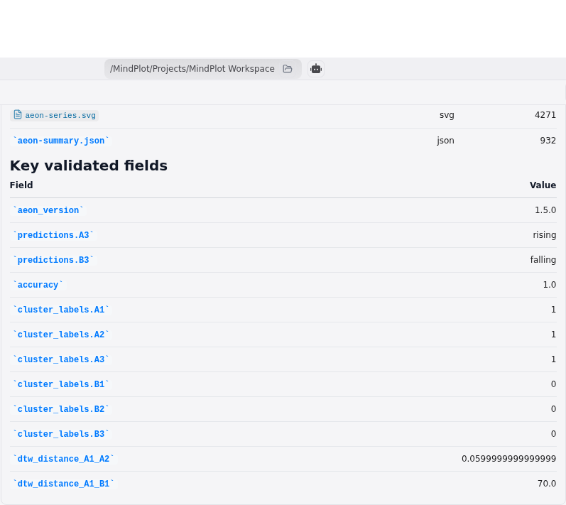
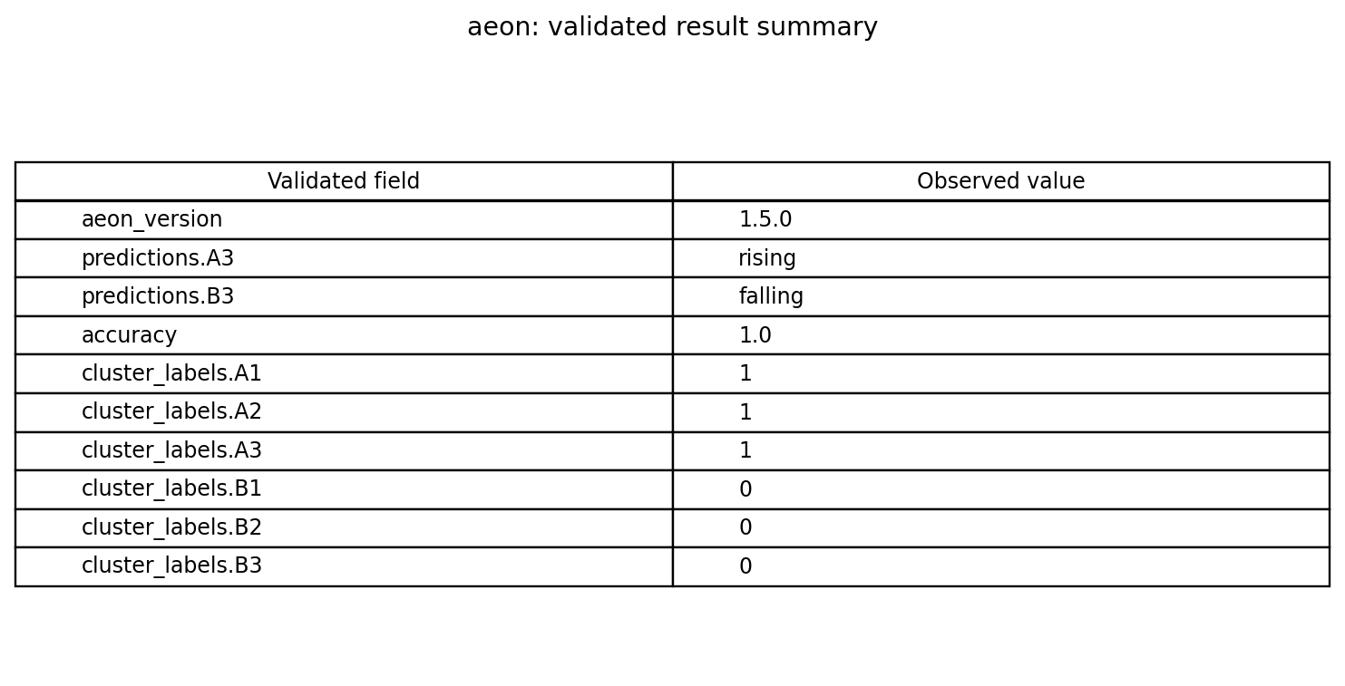
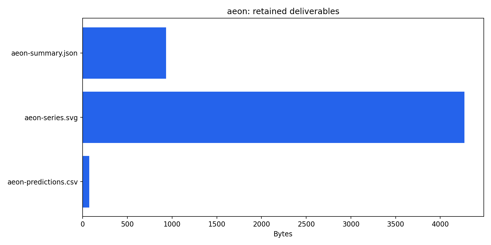
The focused screenshot shows the rendered result rather than an explorer, raw JSON editor, or unrelated application panel. The other two images summarize data-derived values and deliverable provenance. Their SHA-256 digests and sources are recorded in the state manifests.
How to interpret the result
The strongest supported conclusion is narrow: on this deterministic six-series fixture, the installed Aeon version correctly executed the requested whole-series APIs and preserved their results in reusable formats. The large gap between the two DTW comparisons is consistent with the designed patterns. The classification and clustering results agree with the fixture’s construction.
Do not interpret the 1.0 accuracy as a performance claim. There are only two test cases, both are clean synthetic variants, and the analysis did not compare alternative methods. Do not interpret the clusters as discovered biological or physical states. No noise model, measurement process, population, or external validation set was supplied. The SVG is a visual audit aid and not statistical evidence by itself.
For an applied project, begin by defining the prediction unit, target, sampling rate, time origin, channel semantics, and acceptable data leakage boundaries. Split data at the level of independent subjects or acquisition groups. Apply preprocessing inside the training folds. Compare DTW nearest neighbor against simpler and domain-appropriate baselines. Report class-specific metrics and uncertainty. For clustering, assess stability and interpretation rather than selecting the most visually appealing partition.
Reproducibility
Attempt 5 ran on Linux x86_64 with CPU execution, Python 3.11.15, and Aeon 1.5.0. The package and dependencies transferred 142,578,750 bytes. CUDA was neither required nor used. The managed package environment remains under the skill-owned tool directory for inspection and repair, following the retained-environment policy.
To reproduce, preserve the tracked CSV, package pin, input shape, case split, distance choice, random seed, initialization count, and artifact names. Reopen the outputs and assert their content. In particular, verify two prediction rows, exact version 1.5.0, correct within-group cluster membership, distinct groups, ordered DTW distances, and six plotted SVG traces. A later Aeon release or different architecture should be recorded as a new validation environment.
Limitations
This case covers stable core classification, clustering, and distance APIs. It does not validate every estimator or optional dependency in Aeon. It does not cover forecasting, regression, anomaly detection, segmentation, similarity search, deep learning, multivariate scientific data, missing values, irregular sampling, unequal lengths, or very large collections.
The dataset is synthetic, tiny, balanced, equal-length, univariate, and nearly noiseless. Accuracy has no useful precision estimate. The selected DTW values depend on representation and implementation. The clustering repair demonstrates sensitivity to initialization, but the case does not provide a comprehensive stability study. Cross-platform numerical results, especially on macOS ARM, may differ and require their own validation.
References
- Middlehurst et al., “aeon: a Python Toolkit for Learning from Time Series,” Journal of Machine Learning Research, 2024.
- Aeon 1.5.0 installation documentation.
- Aeon time-series classification documentation.
- Sakoe and Chiba, “Dynamic programming algorithm optimization for spoken word recognition,” IEEE Transactions on Acoustics, Speech, and Signal Processing, 1978.
- Aeon package release and Python compatibility metadata.
Try this workflow
MindPlot has built-in support for this scientific skill. You can describe a time-series classification, clustering, or distance-analysis task in ordinary language, attach the dataset, and ask for inspectable tables, JSON summaries, and figures. Users do not need to write or run the Python shown above: the MindPlot agent writes and runs the analysis from the installed skill, then returns the artifacts for review. Try it at mindplot.ai, or download the desktop version for a better experience and stronger local-data privacy.